
Fast and mostly consistent distance field ray marching
Speed limits
In my previous blog post on distance field ray marching, I explained how we can avoid overstepping by making sure that the distance function has gradient magnitude less than 1. This condition is especially useful when we start doing voodoo math adding distance functions together. It gives us a safe “speed limit”.
In this sin noise example, this led me to conclude that I needed to divide the noise component by some factor \( w \) in the distance field \( D(x,y,z) = (1 - ratio) * D_{sphere}(x,y,z) + ratio * D_{noise}(x,y,z) / w \).
However, there is one issue that I swept under the rug. While in theory, you should see rendering artifacts from going above my speed limit, in practice, I need to step as much as 50% faster than the mathematically-derived “speed limit” in order to see any obvious rendering artifacts.
The situation was even worse in another similar demo I created:
In the demo above, instead of adding sin noise (which is too regular) to the distance function of a sphere, I add Perlin noise to the distance function of a sphere. Perlin noise is a commonly used random function that has some smoothness to it. Using numerical optimization, I previously calculated the maximum gradient of 3D Perlin noise to be around 2.793. But in this case, I need to step almost 3x more than my “speed limit” allows to see obvious rendering artifacts.
So this “speed limit” seems rather unconvincing in practice. What’s wrong?
Rare extreme cases
It all comes down to the likelihood of overstepping past the surface of an object when sampling the distance field. One way to get a sense of that is to use a Monte Carlo simulation. First, I generate 50000 random points on the sin noise function \( \sin(x)\sin(y)\sin(z) \) and calculate the gradient magnitude at each point. Then I plot the probability density function of getting any particular value, as well as the cumulative distribution function, see below:
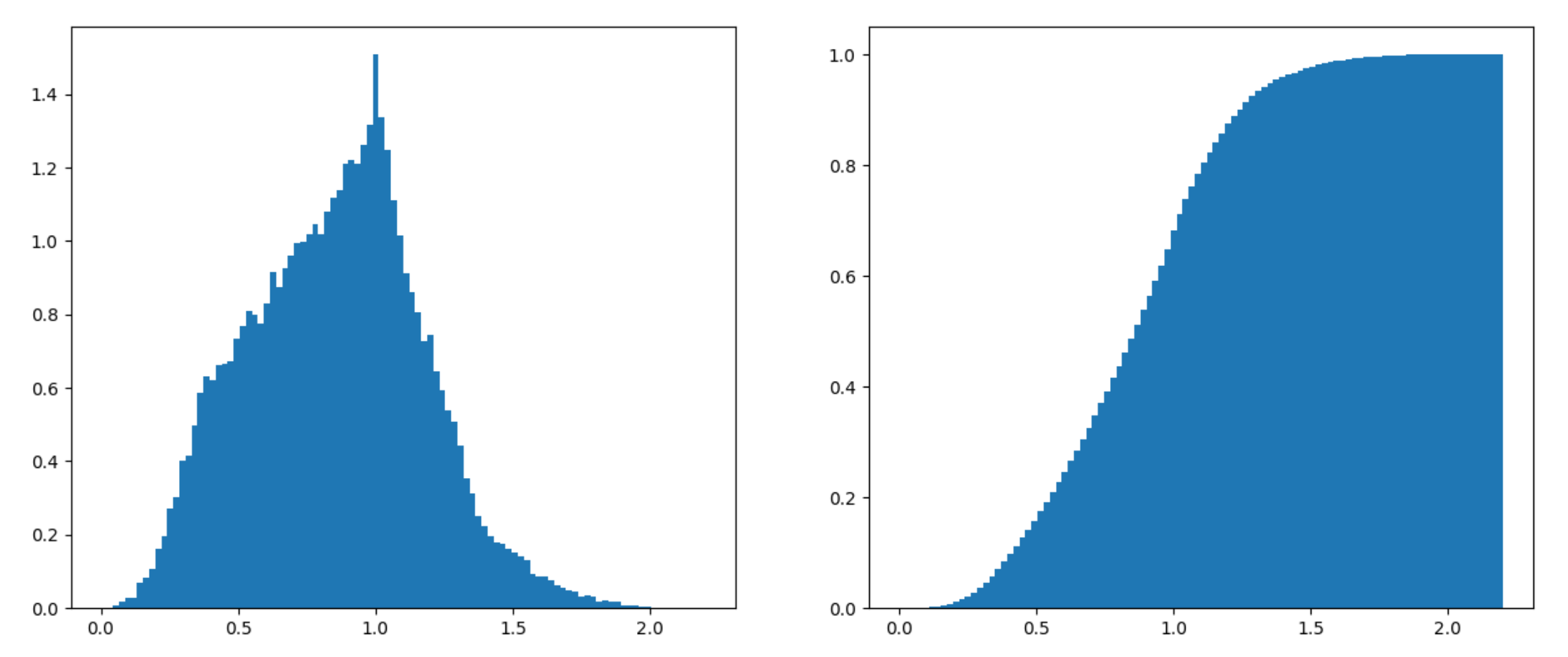
As can be seen, most points will have an average gradient magnitude. The situation is even more extreme with 3D Perlin noise:
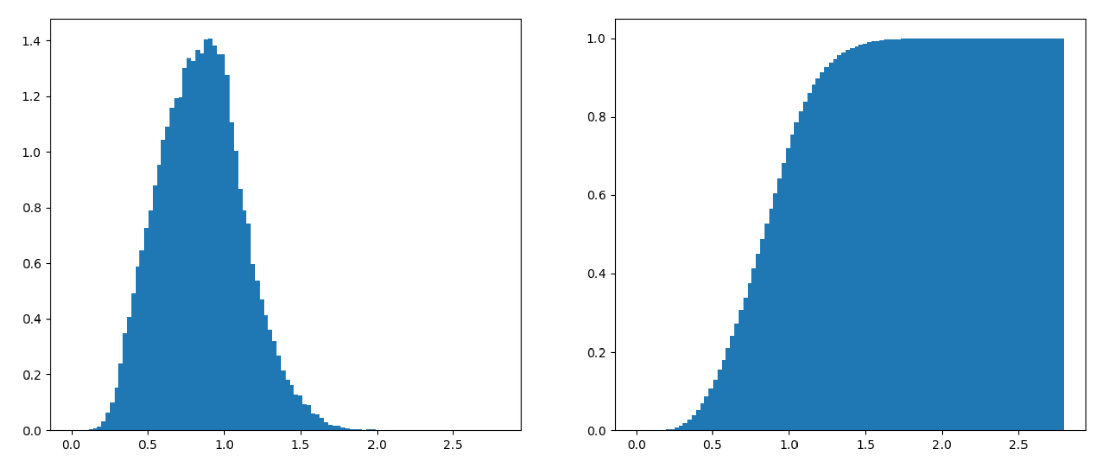
Although we can prove that the gradient of 3D Perlin noise can have a magnitude as large at 2.793, it’s rare that a point will have gradient magnitude more than 1.5, and even rarer that this will cause a rendering artifact. This makes sense. Perlin noise is generated in cubes, each cube being configured via a unit vector at each corner, which can be represented as two angles. In order to hit the worst case, you would need a particular configuration for 16 different variables AND that extreme point would need to be near the surface of the object AND we would need to have a ray pass by that point under a restricted range of angles to see rendering artifacts. Finally, the rendering artifact needs to be significant. If it’s off by only 2-3 values in the RGB spectrum, it’s probably not going to be noticeable.
95th percentile tradeoff
Armed with this knowledge, we can do the following. Instead of using the maximum gradient magnitude as our “speed limit”, we can use the 95th percentile speed limit. That is, pick a value \( x \) such that the gradient magnitude is larger than \( x \) only 5% of the time. In the case of sin noise, this is 0.88. In the case of 3D Perlin noise, this is 1.32.
This is conservative enough that there are no perceptible rendering artifacts, and I only need to go 20-30% faster than my speed limit for there to be clearly visible rendering artifacts.
Smoothly clamped Perlin noise
You might have also read about a modification I made to Perlin noise in order to avoid having to deal with unlikely extreme values. What does the distribution of that Perlin noise look like?
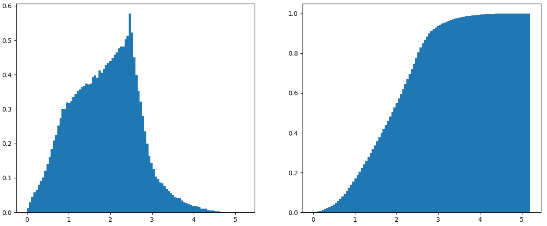
Gradient magnitude PDF and CDF for modified 2D Perlin noise
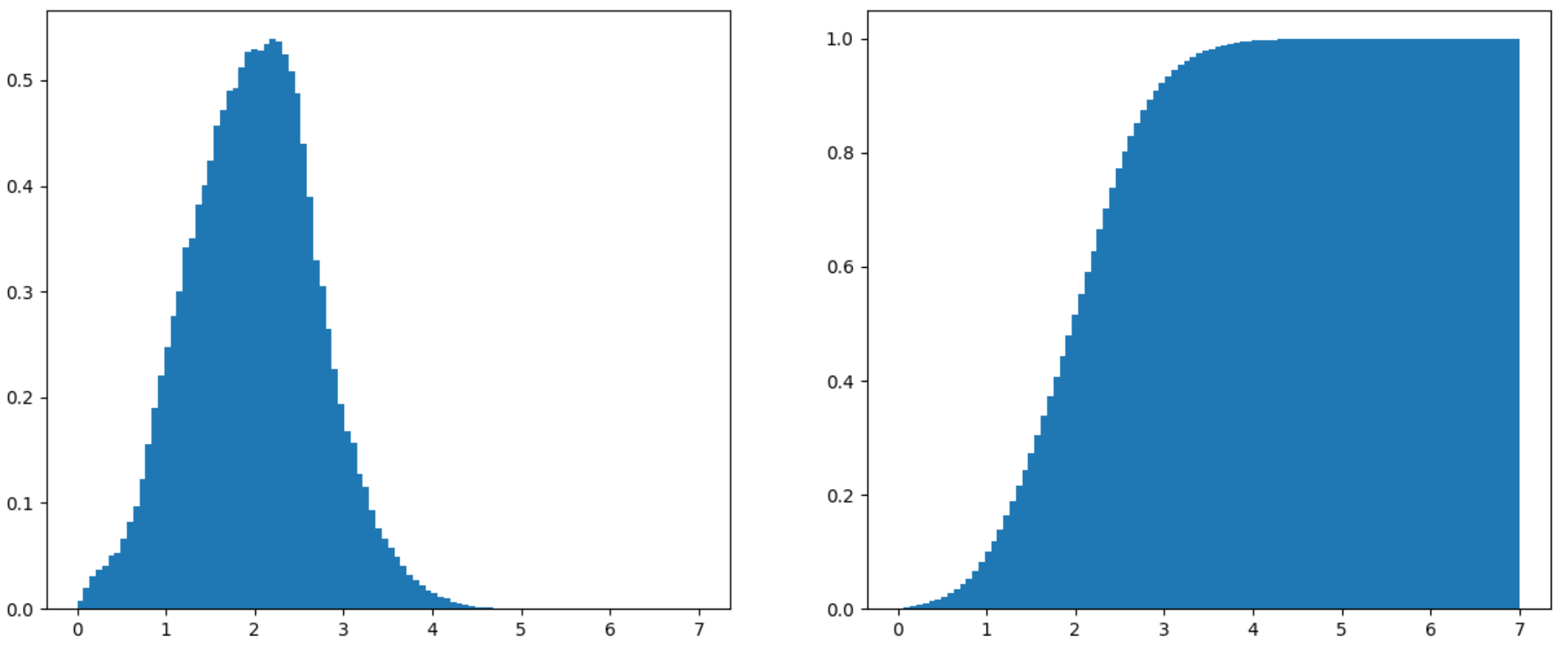
Gradient magnitude PDF and CDF for modified 3D Perlin noise
With a gradient magnitude that goes up to 5.18 and 6.98 respectively, there are also a large range of unlikely gradients. (This Perlin noise is scaled to \( [-1, 1] \), which is why the gradient seems a little large). The 95th percentiles are at 3.12 and 3.18.
So as you can see, efficiently rendering surfaces that are defined by fake distance fields can be quite hard. In these blog posts, I’ve come up with some analysis one can do, but a future goal would be to find more general optimization techniques.
