Restricted Perlin noise for better rendering

In a previous post, I talked about Perlin noise and how it’s important to know the range of values it can take. Today, I want to delve in a little deeper and look at not just the range of values of Perlin noise, but its entire distribution.

Small tail

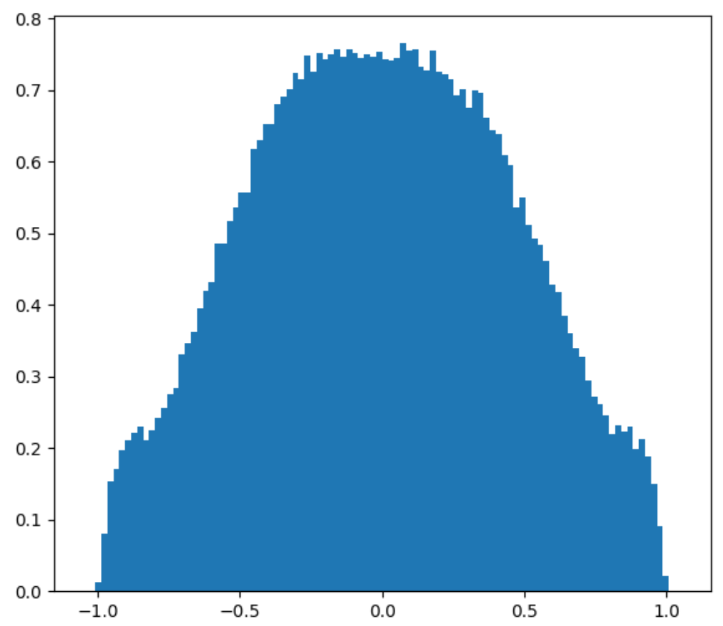
Here’s what happens when you plot the distribution of 2D and 3D Perlin noise using 200 000 stratified random samples, assuming random unit vectors as corner gradients.

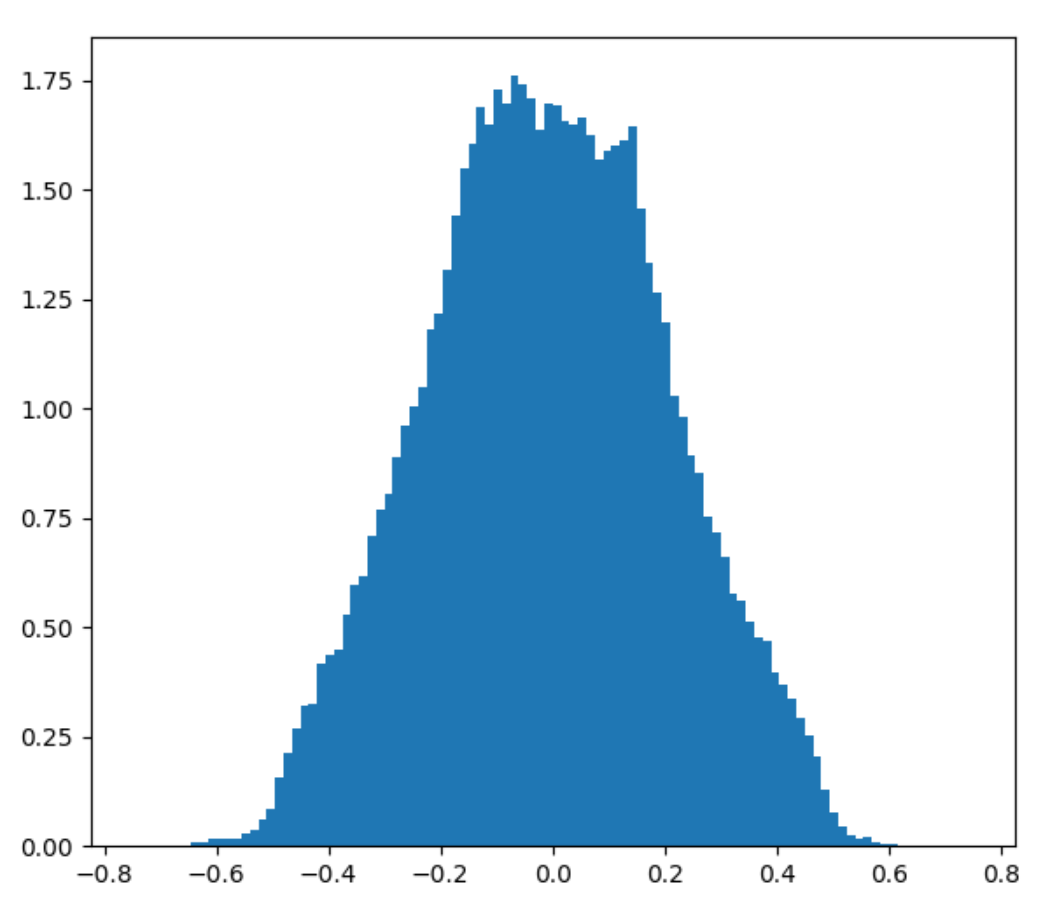
>>> Perlin 2D distribution
Percentile 0: -0.684734
Percentile 2: -0.433033
Percentile 5: -0.364387
Percentile 10: -0.290576
Percentile 20: -0.192601
Percentile 50: -0.004305
Percentile 80: 0.181878
Percentile 90: 0.281137
Percentile 95: 0.358889
Percentile 98: 0.429661
Percentile 100: 0.671943
Mean: -0.004519
Standard deviation: 0.216062

>>> Perlin 3D distribution
Percentile 0: -0.650750
Percentile 2: -0.375985
Percentile 5: -0.312573
Percentile 10: -0.249950
Percentile 20: -0.169677
Percentile 50: 0.002338
Percentile 80: 0.176725
Percentile 90: 0.259164
Percentile 95: 0.322825
Percentile 98: 0.387047
Percentile 100: 0.646493
Mean: 0.003551
Standard deviation: 0.193408

Considering that 2D Perlin has range [-0.707 to 0.707] and 3D Perlin has range [-0.866 to 0.866], we can see from these results that the distribution of Perlin noise values has a tail of possible but highly unlikely values. Even with 200k samples, we didn’t get a single point where the value was above 0.65. As discussed previously, this is because you need to sample Perlin noise in a precise spot under some very small subset of corner gradient configurations to get those extreme values.

Why care

So what if Perlin noise has a tail, do I have a bias against monkeys or something?

The problem is that those extreme values are still possible. This means that in applications where we need to guarantee that the range of values is within [-1, 1], we need to consider the min and max value. However, as they are highly unlikely, in practice we’re generating a random number in a range smaller than [-1, 1]. We lose “contrast”, so to speak.

To be fair, it’s not really that big of a deal. But we can easily fix it with minimal additional compute time, so we might as well.

Removing the tail

The simplest solution would just be to clamp the values. But I wouldn’t be writing a blog post just to tell you to use the clamp function. There are two main issues with clamping:

1) It creates to possibility of flat surfaces (entire areas where the value was clamped). After clamping, the noise function is a mixture of flat and non-flat parts which we do not want to impose on the user. They can decide to flatten areas by clamping themselves if they wish, but that is much easier than unflattening. 2) The derivatives of the function lose continuity and this can lead to sharp edges in the noise. Those sharp edges are visually jarring it creates a discontinuity in the direction of how the light is reflected ¹.

So the thing we need to do is to find a smooth clamping function \( f(x) \) where \( f’(x) \) is continuous. Then we calculate the composition \( f(perlin(\vec{v})) \) which will also have continuous first derivative.

Constructing a smooth clamping function

What properties do we want this function to have?

First, let’s consider only the positive values of Perlin noise (we can deal with the negative values easily since Perlin noise is symmetric around 0). Let’s say that the lower 95% of Perlin noise is in the range \( [0, x_1] \) and the remaining 5% is in the range \( [x_1, x_2] \). We want \( f(perlin(\vec{v})) \) to be smoothly clamped to the range \( [0, p] \).

Define \( q \) to be the proportion of the total range allocated to the lower values (a value between 0.75 and 0.95 is suggested). It would be fair to then map values in the range \( [0, x_1] \) to \( [0, pq] \) and \( [x_1, x_2] \) to \( [pq, p] \). We can do this via two piecewise functions \( f_1, f_2 \). What properties should they have?

The first function \( f_1 \) should pass by \( (x, y) = (0, 0) \) and \( (x, y) = (x_1, pq) \). Although optional, it would be nice if \( f_1’(0) = 1 \) because \( f(x) \) will look like the identity function \( f(x) = x \) at the lowest values. Since we have three constraints, the form of \( f_1 \) should have three parameters, such as a quadratic polynomial ax^2+bx+c.

The second function \( f_2 \) should pass by \( (x, y) = (x_1, pq) \) and \( (x, y) = (x_2, p) \). In order to have continuous derivatives, we would also want \( f_2’(x_1) = f_1’(x_1) \). Finally, it would be nice to have \( f_2’(x_2) = 0 \) as to “tamper off” the function as it reaches the very highest values. It seems that we have four constraints, so it might seem like we would want a cubic polynomial with four degrees of freedom.

Since we have a piecewise polynomial, this looks like a classical spline problem. However, we actually have yet another additional constraint. We need \( f_1(x) <= pq \) for \( x \in [0, x_1] \) and \( f_2(x) \le p \) for \( x \in [x_1, x_2] \). The former is easy to satisfy with a quadratic, but the latter is not because of the higher degree of the polynomial.

Instead, we let \( f_2(x) = d(e-x)^n+g \). That is, we let the degree of the polynomial be a free variable. This form has two advantages. The first is that we can already satisfy two conditions trivially. By having \( f_2(x) = d(x_2-x)^n+p \), we have that \( f_2(x_2) = p \) and \( f_2’(x_2) = 0 \). The second advantage is that \( f_2(x) \) is monotonically increasing on \( [x_1, x_2] \), which will guarantee that \( f_2(x) \le p \).

Now, we can solve for the free variables of \( f_1 \) and \( f_2 \) given those constraints.

Let \( f_1(x) = ax^2 + bx + c, f_1’(x) = 2ax + b \). Since \( f_1(0) = 0 \), then \( c = 0 \). Since \( f_1’(0) = 1 \), then \( b = 1 \). Given those, we can find \( a \) by solving for

\[f_1(x_1) = ax_1^2 + x_1 = qp \implies a = \frac{qp - x_1}{x_1^2}\]

Next, let \( f_2(x) = d(x_2-x)^n+p \). Our two remaining constraints require that \( f(x_1) = d(x_2 - x_1)^n + p = qp \) and \( f’(x_1) = -nd(x_2 - x_1)^{n-1} = f_1’(x_1) \). This gives us that

\[d = \frac{qp - p}{(x_2-x_1)^n} \\ -nd(x_2 - x_1)^{n-1} = -n\frac{qp - p}{(x_2 - x_1)^n}(x_2-n)^{n-1} = -\frac{n(qp - p)}{x_2 - x_1} = f_1'(x_1) \\ n = -(2ax_1 + 1)\frac{x_2 - x_1}{qp - p} \\\]

Putting this all together, we have our smooth clamping function:

\[a = \frac{qp - x_1}{x_1^2} \\ n = -(2ax_1 + 1)\frac{x_2 - x_1}{qp-p} \\ d = \frac{qp - p}{(x_2 - x_1)^n} \\ f(x) = \begin{eqnarray} \left\{ \begin{array}{l} -f(-x) & x < 0 \\ ax^2 + x & x \in [0, x_1] \\ d(x_2 - x)^n+p & x \in [x_1, x_2] \end{array} \right. \end{eqnarray}\]

To get a sense of what (the positive part of) this looks like, I’ve embedded the graph below. If you open it in Desmos, you can also adjust the parameters yourself with a slider and see that our constraints are still satisfied.

What it looks like

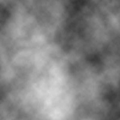
Below is the old Perlin noise and the new Perlin noise, with the same configurations. Unsurprisingly, it looks as if we put the image in Photoshop and increased the contrast.

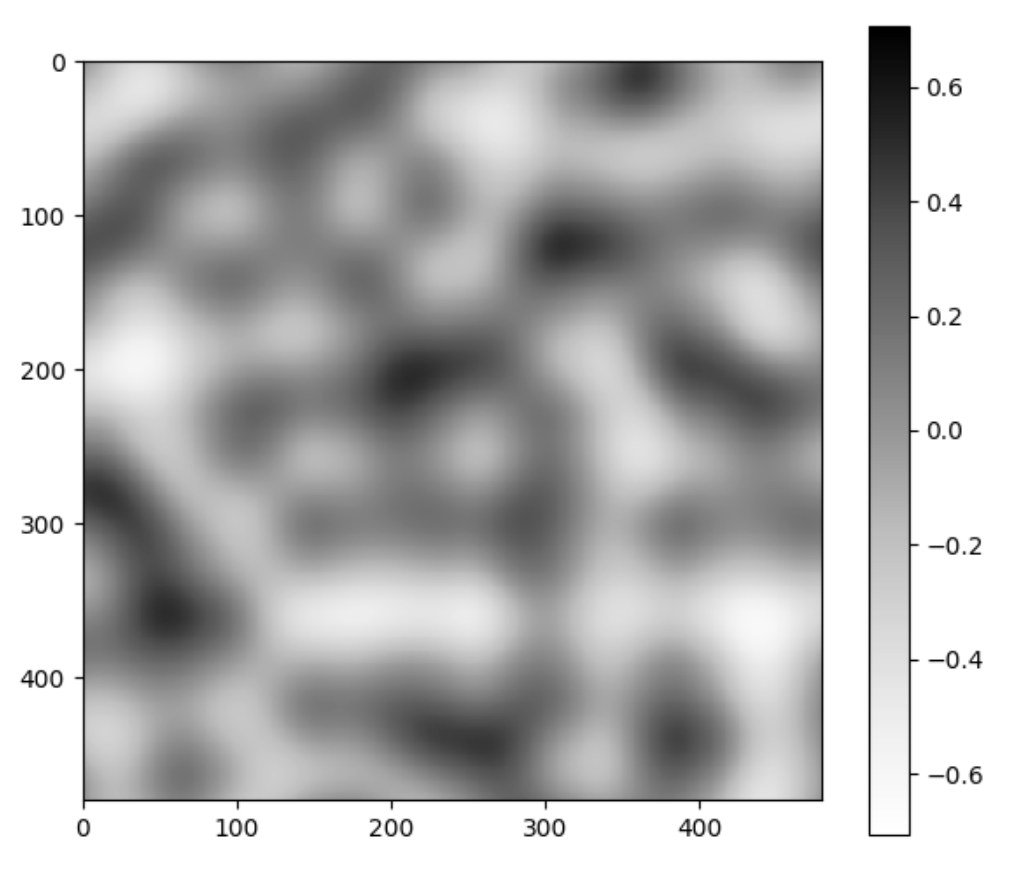
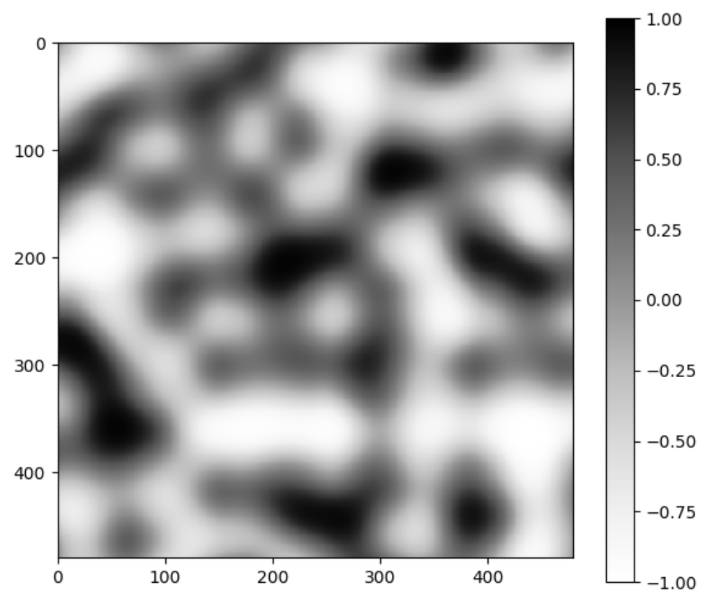
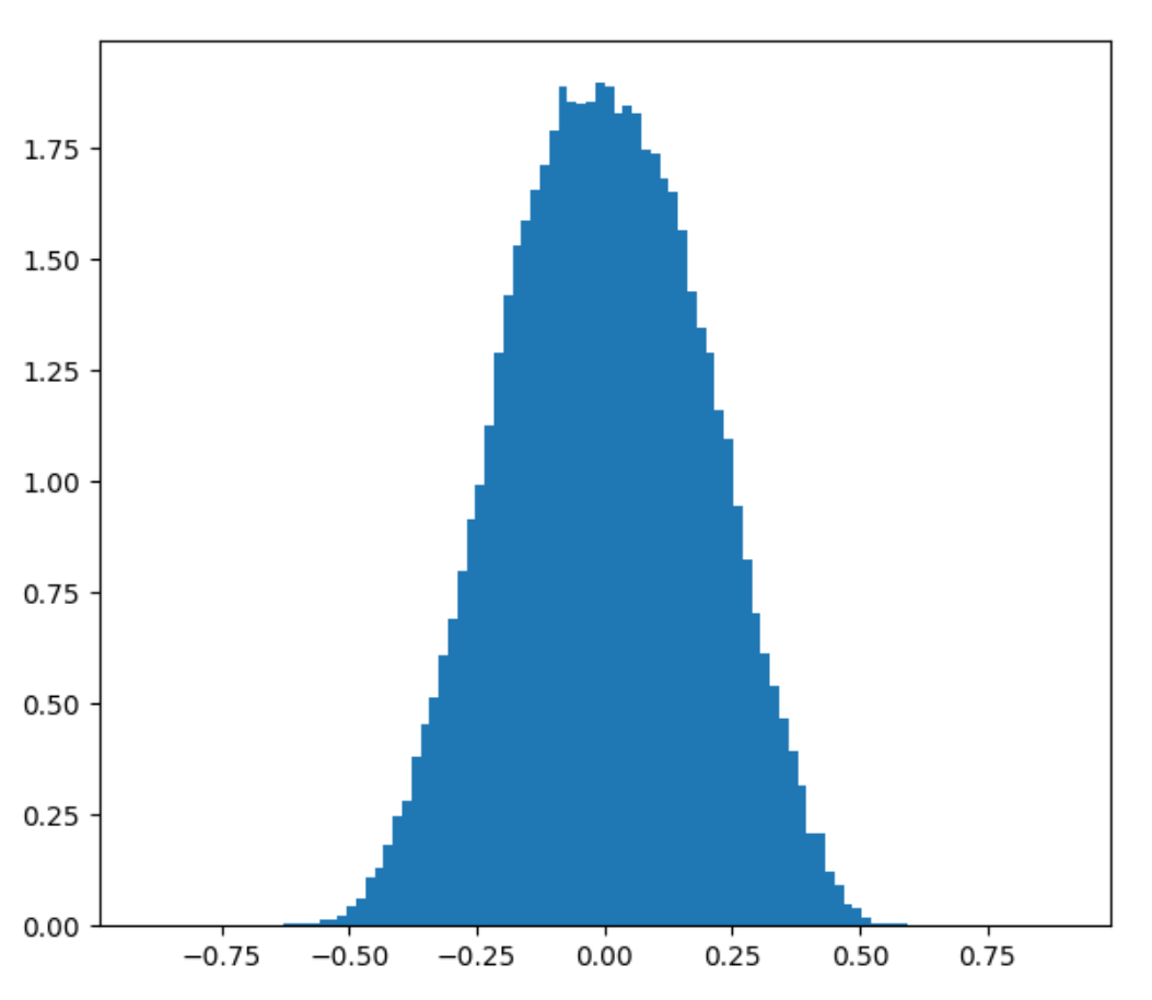
It looks like we have more uniform black and white blobs, at the expense of the grays. This is mostly due to human perception. If we plot the distribution of this new noise function, we still get that greys are the dominant color, but there are a lot more blacks and whites now.

PDF of new 2D and 3D Perlin noise

A lot of the code used to make these plots can be found on my Github.

Multiple octaves of Perlin noise

So now we’ve got a useful modification to Perlin noise, but people rarely use plain Perlin noise in their applications. More commonly, people will sum up different frequencies of Perlin noise together to get a fractal-like texture that has detail at multiple different resolution levels. For example, this is often used to generate clouds or heightfields.

Sum of Perlin noise at different frequencies

As a side effect of summing up different Perlin noises, we also create a longer tail. That is, we get even bigger min and max values that are even less likely to show up. To get an intuition for this, think about how each roll of a 6-sided dice has equal probability. Now, think about the probability of getting a particular sum when rolling two 6-sided dices . You’ve probably learned before that rolling a 7 is the most likely outcome, because 7 is right in the middle. It’s 6 times more likely than rolling a 2 or a 12. Similarly, when you sum up two Perlin noises, you need both of them to have their most extreme configuration and align them in such a way that the maximum point of both end up at the same point. Only then do you get the maximum value of the sum of two Perlin noises!

So trimming the tail is even more important when it comes to the sum of Perlin noise functions.

Finding out the size of the tail

We could do the same thing we’ve done before with plain Perlin noise to find the distribution of the sum of Perlin noises: do lots of simulations. However, this is going to become unwieldy rather quickly. There’s infinitely many ways to sum up Perlin noise at different frequencies (by assigning different weights), and we don’t want to have to do a simulation every time. It takes a lot of time to generate enough samples.

Instead, let’s come up with a simple formula that we can use. I said in the previous blog post that Perlin noise is not Gaussian-distributed. That’s true, but it does have the shape of a bell curve, at least enough that approximating it with a Gaussian would be reasonable.

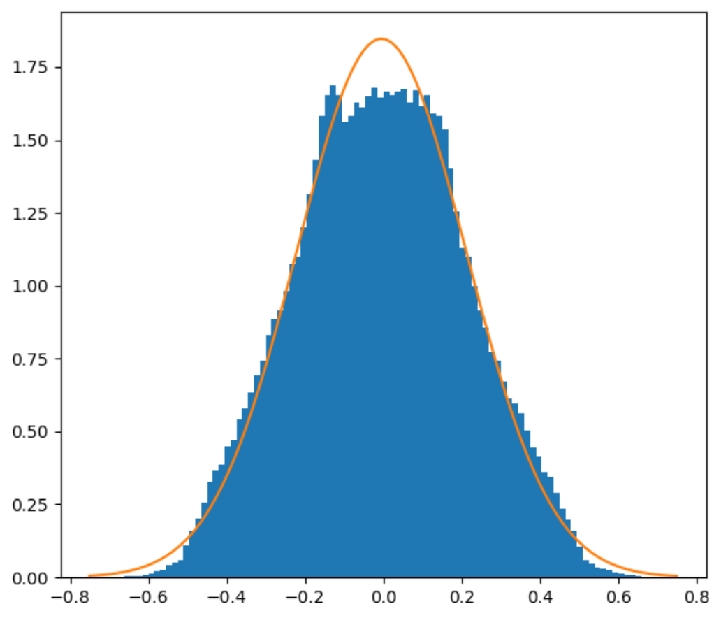
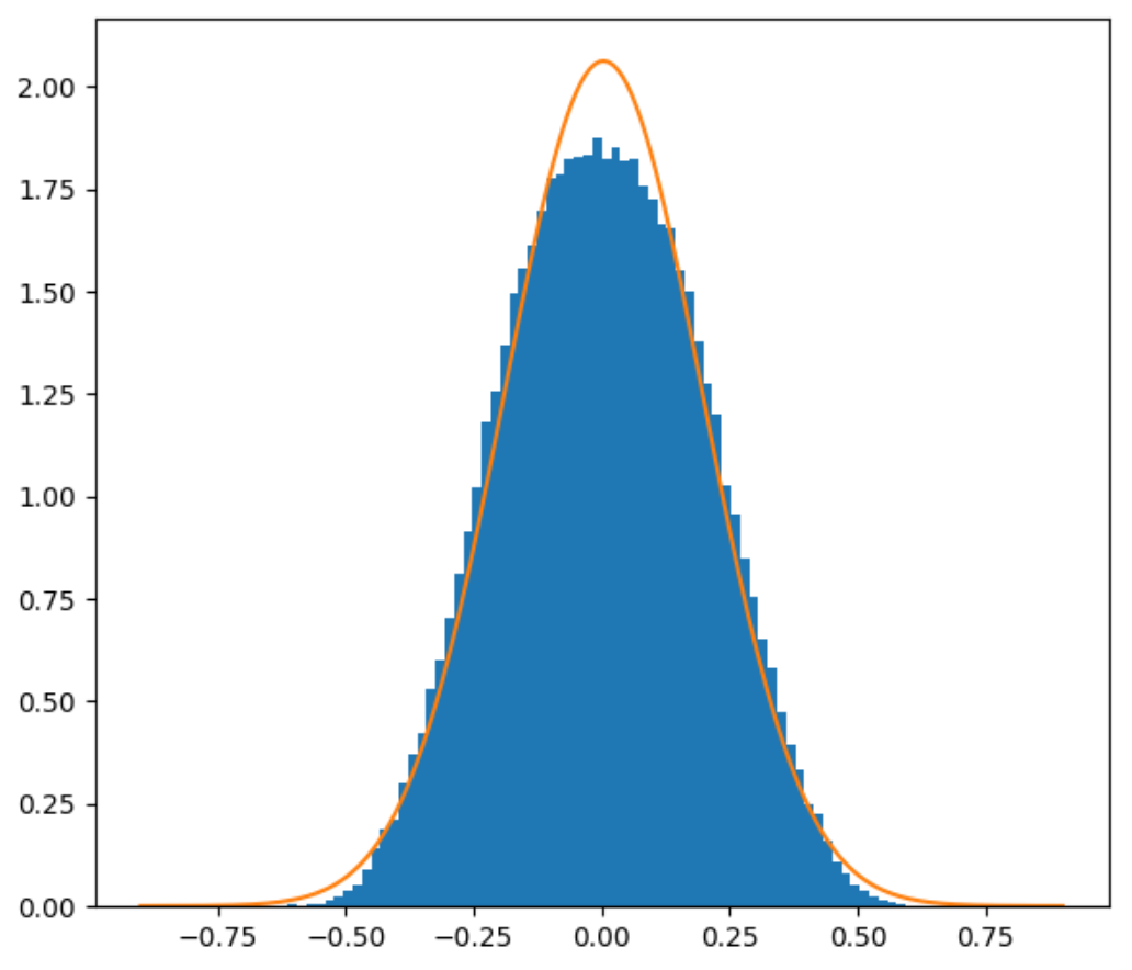
2D and 3D Perlin noise PDFs with Gaussian approximation

Gaussians have some nice properties that can help us here. Normally, when you want to compute the PDF of \( Z = X + Y \) where \( X, Y \) are random variables with known PDFs, you have to take the convolution between the PDFs of \( X \) and \( Y \), which is an expensive operation (\( O(n^2) \) naively, \( O(n\log{n}) \) with heavy machinery like fourier transforms). However, summing up Gaussians is really easy. If \( X, Y \) are Gaussians-distributed with mean \( \mu_x, \mu_y \) and variance \( \sigma_x^2, \sigma_y^2 \), then the resulting random variable \( Z = X + Y \) is a gaussian with mean \( \mu_x + \mu_y \) and variance \( \sigma_x^2 + \sigma_y^2 \).

Furthermore if we set our smooth clamping threshold to \( 2\sigma \), then we get rid of approximately 5% of extreme values, which seems reasonable.

That was a lot of work…

…for what seems like a rather pedantic little detail. And in most cases, it will be. All the additional complexity to smoothly clamp large values of the Perlin noise exists to avoid some occasional visual artifacts, but the world of computer graphics is already quite tolerant of “good enough”. However, in some cases where it’s nice to have guarantees, like with distance field ray marching, this work can hopefully be useful.

---