Consistent distance fields for ray marching

Introduction

The classical way of writing a ray tracer represents objects in your scene with a triangle mesh. You then shoot some light rays out of your camera and do some algebra to see if it intersects with any triangles.

In recent years, an alternative to triangle-based ray tracing has emerged. While slightly less general, it’s fast enough to ray-trace scenes in real-time. It’s been popular in the hobbyist community for being able to produce cool results with few lines of code. The key is to use something called a “distance field”.

A distance function \( D(x,y,z) \) tells you, for any point \( (x,y,z) \) in space, how far the closest object is. It doesn’t tell you what direction, just the distance to the closest object. Using such a function, however, makes ray marching really easy. You start the ray at the position of the camera. You calculate \( d = D(x,y,z) \). This tells you that you can move the ray forward by distance \( d \) without hitting any object. Repeat this process until you get within some epsilon distance of the object.

The code for this process is equally simple:

float castRay(vec3 pos, vec3 rayDir) {
    float dist = 0.0;

    for (int i = 0; i < ITERATIONS; i++)
    {
        float res = distanceFn(pos + rayDir * dist);
        if (res < EPSILON || dist > MAX_DIST) break;
        dist += res;
    }

    return dist;
}

How do you find these distance functions? Constructing them for some primitives is very simple. Here is a sphere and the distance function of a sphere:

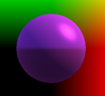
float distanceSphere(vec3 pos, float radius)
{
    return length(pos) - radius;
}

You can find many more examples of primitive shapes, as well as how to combine them and modify them, on Inigo Quilez’s website.

It can be difficult, however, to create distance functions for complex shapes using only primitive operations. What people will often do in practice is to create functions that give you an estimate of the distance to the closest object. But regardless of the nature of the estimate, points where the distance function \( d(x, y, z) = 0 \) represent the surface of the object (think for a second why this is true).

For example, I’ve obtained the funky-looking shape on the left by using the distance function the right.

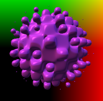
float distanceFunkySphere(vec3 pos, float radius, float frequency)
{
    float noise = sin(pos.x*frequency)*sin(pos.y*frequency)*sin(pos.z*frequency);
    return length(pos) - radius + noise;
}

Where the original distanceSphere function gave me the exact distance to the closest object, the new distanceFunkySphere function doesn’t do that. It gives me an estimate to the distance of some surface (that’s no longer just a sphere). But my ray marching code never needed the exact distance to begin with, since it gets closer to the surface step by step.

Finally, you can render this super fast because each of these ray marching procedures on distance functions can be evaluated independently for each pixel on the screen (you just change the ray direction). This is the kind of work that the GPU is best at!

If this is new to you so far and you find this interesting, I recommend taking a look at cool demos on Shadertoy and exploring Inigo Quilez’s website who gets a lot of credit for popularizing this technique. If you’re already familiar with distance field ray marching, read on, as I’m going to get into some technical details that are important for producing good distance functions.

Overstepping

In the example above, I multiplied some sin functions and added it to a distance function of a sphere to get a sphere with bubbles. If you’re acquainted with the hobbyist community that uses distance functions, something about it should feel familiar. You do some random math operations, get something physically incorrect, stick in some arbitrary constants for adjustment, wave your hands and say “hey, the result looks nice!”.

A friend of mine, Veit Heller coined a good term for this: voodoo math.

Getting a physically incorrect result isn’t always a problem. You could, for example, divide a distance function by 2. It’ll never answer the question “how far is the closest point?” correctly, but at worst it’ll take twice as many steps for ray marching to hit the surface of the object.

Problems occur when your distance function gives you a result that’s too large. Then you might take a ray marching step past the surface of your object.

This kind of overstepping will either fail to render thin objects (jump past it) or render the inside of an object, leading to weird results.

To see how this is important, consider the animation below. On the left side, I’m ray marching 25% faster than the safe “speed limit” (more on that in a second). On the right side, I have the reference, correct image. If you squint your eyes and look carefully at the surface as it’s moving, you should see some “ripples” that appear at random times. That’s caused by overstepping.

I used this particular shape as an example since it’s used in the primitives demo. I noticed that the rippling happens as the object gets close to the camera.

Preventing overstepping

How do you guarantee that overstepping won’t happen? A useful heuristic is to look at how fast the function changes. If the magnitude of the gradient of the function is less or equal to one everywhere that it’s defined, then you will never overstep.

To get an intuition of how this is true, consider the one-dimensional case, where \( D(x) \) is the distance to a point at \( x = 0 \). Then the line \( D(x) = x \) is the maximum allowed value of \( D(x) \) and has gradient (derivative) equal to 1 everywhere except at \( x = 0 \) where it’s not defined. If the gradient can only be smaller, \( D(x) \) can also only be smaller.

This is a rather strong condition. You could have functions that are consistent distance fields (that do not overstep) and that have a large gradient in some small area that doesn’t matter, like the one below.

In that case, dividing by the gradient magnitude would be unnecessarily conservative. However, if we start adding it to other distance functions, than that small area with large gradient suddenly starts to matter.

In the case of our sin noise function, that is what we do.

Anyway, what is the gradient of our noise function? Recall that it’s defined as:

Then \( \nabla n = (w\cos{wx}\sin{wy}\sin{wz}, w\sin{wx}\cos{wy}\sin{wz}, w\sin{wx}\sin{wy}\cos{wz}) \). Next we find an upper bound for the gradient magnitude.

So the gradient of \( n(x, y, z) \) is at most \( w \), the noise frequency. That means that \( \frac{n(x,y,z)}{w} \) is a distance function guaranteed not to overstep.

But wait, the distance function that we used was \( D(x,y,z) = D_{sphere}(x,y,z) + D_{noise}(x,y,z) \)!

The gradient of \( D_{sphere} \) is exactly 1 everywhere (exercise for the reader - this is also true for all exact distance functions). We can use the triangle inequality to get that \( \norm{\nabla D(x,y,z)} <= \norm{\nabla D_{sphere}(x,y,z)} + \norm{\nabla D_{noise}(x,y,z)} = 1 + w \). So it suffices to divide \( D(x,y,z) \) by \( (1 + w) \). Now, using that distance function, we are guaranteed not to overstep.

In practice, we adjust the strength of the noise component by using linear interpolation \( D(x,y,z) = (1 - ratio) * D_{sphere}(x,y,z) + ratio * D_{noise}(x,y,z) / w \). In GLSL, this can be done with the mix function.

Useful properties of gradients and gradient maximums

Linearity: \( \nabla(\alpha F(\vec{v}) + \beta G(\vec{v})) = \alpha \nabla F(\vec{v}) + \beta \nabla G(\vec{v}) \)

Product rule: \( \nabla(F(\vec{v}) G(\vec{v})) = F(\vec{v}) \nabla G(\vec{v}) + G(\vec{v}) \nabla F(\vec{v}) \)

Chain rule: \( \nabla(g(F(\vec{v}))) = g’(F(\vec{v})) \nabla F(\vec{v}) \)

Minimum: \( \nabla (\min(F(\vec{v}), G(\vec{v}))) \le \max(\nabla F(\vec{v}), \nabla G(\vec{v})) \)

Maximum: \( \nabla (\max(F(\vec{v}), G(\vec{v}))) \le \max(\nabla F(\vec{v}), \nabla G(\vec{v})) \)

Absolute value: \( \nabla (abs(F(\vec{v}))) = \nabla F(\vec{v}) \).

Triangle inequality: If \( \vec{a} = \vec{b} + \vec{c} \), then \( \norm{\vec{a}} \le \norm{\vec{b}} + \norm{\vec{c}} \).

Fast ray marching

The method we used to find a scaling factor for our distance function uses the maximum of the magnitude of the gradient as well as the triangle inequality. It gives us a conservative estimate, based on the potential worst cases. This means that we are probably overestimating the scaling factor and marching slower than we need to. Can we do better? See my next blog post.